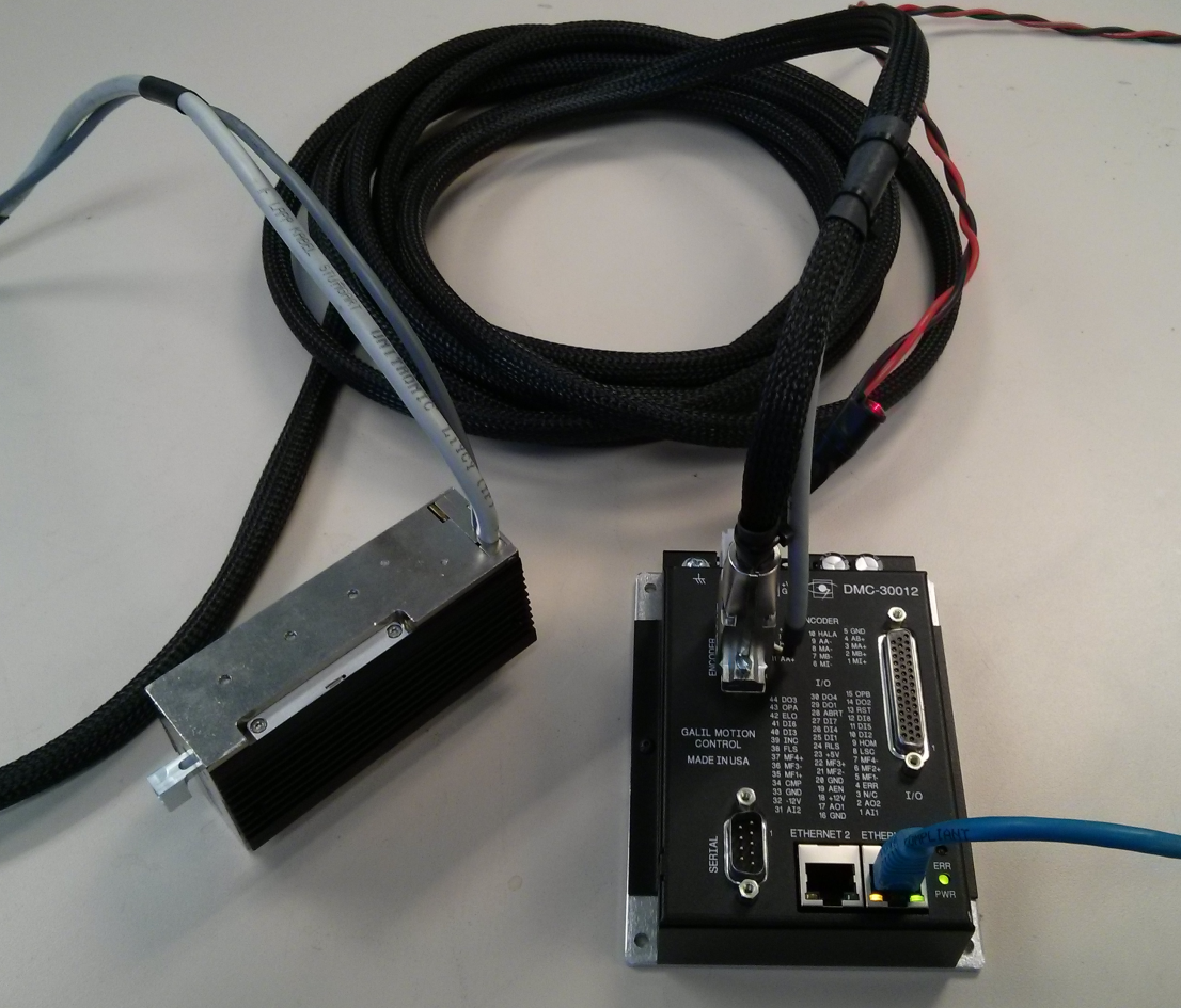
Customer’s needs for servo control has progressed over the years resulting in more exotic mechanics being introduced into the market. Examples of some of these new mechanics are nonlinear systems such as articulated arms and spring-based mechanisms.
Nonlinear systems introduce forces that are not uniform into the control system. These non-uniform forces must have compensation. Compensating for a uniform force, such as gravity, is simple because you can add force to directly compensate for the force of gravity. Compensating for a force that isn’t uniform can be complicated because of its dynamic nature. For example, an articulating arm has the force from gravity added to the load while the arm is horizontal, but no additional force from gravity when the arm is vertical. The length of the arm also affects the load. The additional load seen by the arm can be calculated by using sin(rQ)*F where r is the arm length, Q is the angle, and F is the force from gravity.
A spring mounted to a stage will have similar forces added to the load but the motor/spring position will be the driving force of the equation instead of the angle. The equation to calculate the force, or compensation, for a spring is y=mx+b, where y is the force, x is the motor position, m is the spring constant (in terms of volts/count), and b is the spring preloading. The picture below shows an application that uses a SMAC linear motor, that is connected to internal spring and has 1 micron resolution, connected to a Galil DMC-30012 (controller and amplifier).
| Command | Description |
|---|---|
| #f | Beginning of loop |
| OFA=(m*_TPA/scale)+b+vertoff | calculate force/offset on axis A, vertoff used if vertical axis |
| WT 2 | GalilSuite Scope View of Settling Time |


